-
PRODUCTS & SERVICESOptimized cooling solutions for modern data centersProducts & ServicesOptimized cooling solutions for modern data centers
-
CAPABILITIESAdvancing liquid cooling technologiesCapabilitiesAdvancing liquid cooling technologies
-
TechnologiesLiquid Cooling InnovationTechnologiesLiquid Cooling Innovation
-
RESOURCESLatest News & InformationResourcesLatest News & Information
-
ABOUTOur history, leadership and ownershipAboutOur history, leadership and ownership
-
CONTACTFacility locations and global operational footprint





7 Tips for Buying Confocal Raman Spectroscopy Systems?
Buying a Confocal Raman Spectroscopy system is not simply a matter of comparing laser wavelengths and detector prices. The right instrument must fit your samples, workflow, room, and long-term research goals. A polished demonstration can look impressive. Real performance may feel different beside a crowded laboratory bench.
Professor Peter L. McCreery, a respected Raman spectroscopy authority, has stated, “Raman spectroscopy provides molecular information without destroying the sample.” That principle remains valuable, but purchasing decisions require more than non-destructive analysis. You must examine signal strength, spectral resolution, confocal performance, fluorescence rejection, software usability, and service support. Small details matter. A weak signal at 785 nanometers may become frustrating during a late-night measurement.
This guide presents seven practical tips for buying a Confocal Raman Spectroscopy system. It considers application requirements before technical specifications. It also explains how to compare lasers, microscopes, sample stages, calibration routines, and safety features. Experience shows that the most expensive system is not always the most suitable one. That is worth remembering.
Ask difficult questions. Test real samples. Request raw spectra, not only colorful images. Check whether the supplier can measure your thick, dark, transparent, or heat-sensitive materials. One limitation should be admitted: no short guide can replace an on-site evaluation. Still, a careful checklist can prevent costly assumptions. The goal is a reliable system that produces interpretable data repeatedly, not merely an impressive demonstration on one ideal sample.
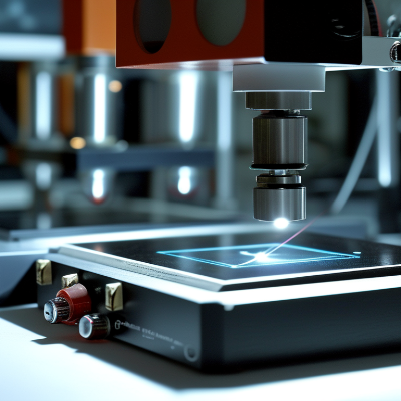
Table of Contents [Hide]
Define Confocal Raman Spectroscopy and Its Core Applications
Confocal Raman spectroscopy combines Raman scattering with optical sectioning. A focused laser illuminates a tiny region, while the spectrometer records wavelength shifts from molecular vibrations. A confocal pinhole rejects much of the out-of-focus signal. This creates sharper chemical images and supports depth analysis. It is not magic. Signal strength still depends on material, surface quality, laser wavelength, and exposure time.
The technique helps identify unknown compounds without cutting samples. In a polymer cross-section, it can reveal layers only a few micrometres apart. In a mineral grain, Raman peaks can distinguish phases that look identical under ordinary light. Researchers also use it for pharmaceutical screening, semiconductor inspection, biological samples, pigments, and corrosion studies. Mapping can show where a component sits, while depth scans can expose contamination below a surface.
When assessing a system, match its capabilities to the sample rather than choosing specifications alone. Check spectral resolution, spatial resolution, laser options, detector sensitivity, calibration stability, and confocal performance. Fluorescence may overwhelm Raman signals, especially in organic or aged materials. Lower laser power can protect delicate samples, but measurements may take longer. A practical test with your own sample is often more revealing than a polished demonstration. The clearest image is not always the most reliable result. Poor focusing, weak calibration, or aggressive processing can create convincing but misleading maps. Depth matters.